5/27/2009

05-27-09 - Optimal Local Bases

I've had this idea forever but didn't want to write about it because I wanted to try it, and I hate writing about things before I try them. Anyway, I'm probably never going to do it, so here it is :

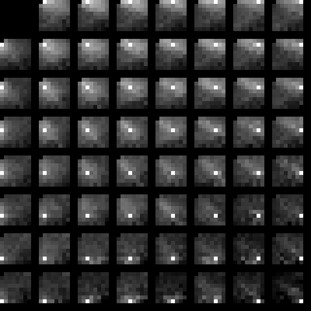
It's obvious that we are now at a point where we could use the actual optimal KLT for 4x4 transforms. That is, for a given image, take all the 4x4 blocks and turn them into a 16-element vector. Do the PCA to find the 16 bases vectors that span that 16-element space optimally. Tack those together to make a 16x16 matrix. This is now your KLT transform for 4x4 blocks.

(in my terminology, the PCA is the solve to find the spanning axes of maximum variance of a set of vectors; the KLT is the orthonormal transform made by using the PCA basis vectors as the rows of a matrix).

BTW there's another option which is to do it seperably - a 4-tap optimal horizontal transform and a 4-tap optimal vertical transform. That would give you two 4x4 KLT matrices instead of one 16x16 , so it's a whole lot less work to do, but it doesn't capture any of the shape information in the 2d regions, so I conjecture you would lose almost all of the benefit. If you think about, there's not much else you can do in a 4-tap transform other than what the DCT or the Hadamard already does, which is basically {++++,++--,-++-,+-+-}.

Now, to transform your image you just take each 4x4 block, multiply it by the 16x16 KLT matrix, and away you go. You have to transmit the KLT matrix, which is a bit tricky. There would seem to be 256 coefficients, but in fact there are only 15+14+13.. = 16*15/2 = 120. This because you know the matrix is a rotation matrix, each row is normal - that's one constraint, and each row is perpendicular to all previous, so the first only has 15 free parameters, the second has 14, etc.

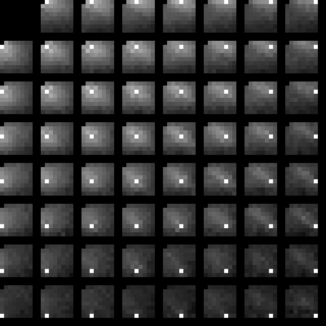
If you want to go one step crazier, you could do local adaptive fitting like glicbawls. For each 4x4 block that you want to send, take the blocks in the local neghborhood. Do the PCA to find the KLT, weighting each block by its proximity to the current. Use that optimal local KLT for the current block. The encoder and decoder perform the same optimization, so the basis vectors don't need to be transmitted. This solve will surely be dangerously under-conditioned, so you would need to use a regularizer that gives you the DCT in degenerate cases.

I conjecture that this would rock ass on weird images like "barb" that have very specific weird patterns that are repeated a lot, because a basis vector will be optimized that exactly matches those patterns. But there are still some problems with this method. In particular, 4x4 transforms are too small.

We'd like to go to 8x8, but we really can't. The first problem is that the computation complexity is like (size)^8 , so 8x8 is 256 X slower than 4x4 (a basis vector has (size^2) elements, there are (size^2) basis vectors, and a typical PCA is O(N^2)). Even if speed wasn't a problem though, it would still suck. If we had to transmit the KLT matrix, it would be 64*63/2 = 2016 coefficients to transmit - way too much overhead except on very large images. If we tried to local fit, the problem is there are too many coefficients to fit so we would be severely undertrained.

So our only hope is to use the 4x4 and hope we can fix it using something like the 2nd-pass Hadamard ala H264/JPEG-XR. That might work but it's an ugly heuristic addition to our "optimal" bases.

The interesting thing about this to me is that it's sort of the right way to do an image LZ thing, and it unifies transform coding and context/predict coding. The problem with image LZ is that the things you can match from are an overcomplete set - there are lots of different match locations that give you the exact same current pixel. What you want to do is consider all the possible match locations - merge up the ones that are very similar, but give those higher probability - hmmm.. that's just the PCA!

You can think of the optimal local bases as predictions from the context. The 1st basis is the one we predicted would have most of the energy - so first we send our dot product with that basis and hopefully it's mostly correct. Now we have some residual if that basis wasn't perfect, well the 2nd basis is what we predicted the residual would be, so now we dot with that and send that. You see, it's just like context modeling making a prediction. Furthermore when you do the PCA to build the optimal local KLT, the eigenvalues of the PCA step tell you how much confidence to have in the quality of your prediction - it tell you what probability model to use on each of the coefficients. In a highly predictable area, the 1st eigenvalue will be close to 100% of the energy, so you should code predicting the higher residuals to be zero strongly; in a highly random area, the eigenvalues of the PCA will be almost all the same, so you should expect to code multiple residuals.

5/26/2009

05-26-09 - Some Study of DCT coefficients

First of all : The number of non-zero values in the lower-diagonal area of the 8x8 block after quantization to a reasonable/typical value.

(36 of the 64 values are considered to be "lower diagonal" in the bottom right area) The actual number :


avg : 3.18 : 
 0 : 37.01
 1 : 16.35
 2 :  9.37
 3 :  6.48
 4 :  5.04
 5 :  3.88
 6 :  3.22
 7 :  3.02
 8 :  2.49
 9 :  2.34
10 :  2.09
...

The interesting thing about this is that it has a very flat tail, much flatter than you might expect. For example, if the probability of a given coefficient being zero or nonzero was an indepedent random event, the distribution would be binomial; it peaks flatter and is then much faster to zero :

avg : 3.18 : 
 0 : 13.867587
 1 : 28.162718
 2 : 27.802496
 3 : 17.775123
 4 : 8.272518
 5 : 2.986681
 6 : 0.870503
 7 : 0.210458
 8 : 0.043037
 9 : 0.007553
10 : 0.001150
...

What this tells us is the probability of a given coefficient being zero is highly *not* idependent. They are strongly correlated - the more values that are on, the more likely it is that the next will be on. In fact we see that if there are 6 values on, it's almost equally likely there are 7, etc. , that is : P(n)/P(n-1) goes toward 1.0 as n gets larger.

Also, amusingly the first two ratios P(1)/P(0) and P(2)/P(1) are both very close to 0.5 in every image I'm tried (in 0.4 to 0.6 generally). What this means is it wouldn't be too awful just to code the # of values on with unary, at least for the first bit (you could use something like an Elias Gamma code which uses unary at first then adds more raw bits).

Now for pretty pictures. Everyone has seen graphics like this, showing the L2 energy of each coefficient in the DCT : (none of these pictures include the DC because it's weird and different)

This shows the percentage of the time the value is exactly zero :

Now for some more interesting stuff. This shows the percent of correlation to the block above the current one : (to the north) :

Note in particular the strong correlation of the first row.

The next one is the correlation to the block to the left (west) :

Finally the fun one. This one shows the correlation of each coefficient to the other 63 coefficients in the same block :

The self-correlation is 100% which makes it a white pixel obviously. Black means 0% correlation. This is absolute-value correlation in all cases (no signs). There are a lot of patterns that should be pretty obvious to the eye. Beware a bit in over-modeling on these patterns because they do change a bit from image to image, but the general trend stays the same.

And another one from a different image :

This one's from Lena. A few things I think are particularly interesting - in the upper left area, which is where most of the important energy is, the correlation is most strong diagonally. That is, you see these "X" shape patterns where the center pixel is correlated mainly to it's diagonal neighbors, not the one's directly adjacent to it.

05-26-09 - Storing Floating Points

I rambled a bit before about how to store floating point images . I think I have the awesome solution.

First of all there are two issues :

Goal 1. Putting the floating point data into a format that I can easily run through filters, deltas from previous, etc. Even if you're doing lossless storage your want to be able to delta from previous and have the deltas make sense and preserve the original values.

Goal 2. Quantizing in such a way that the bits are used where the precision is wanted. Obviously you want to be sending bits only for values that are actually possible in the floating point number.

Also to be clear before I start, the issue here is with data that's "true floating point". That is, it's not just data that happens to be in floating point but could be equally well converted to ints inside some [min,max] range. For example, the coordinates of most geometry in video games really isn't meant to be floating point, the extra precision near zero is not actually wanted. The classic example where you actually want floating point is for HDR images where you want a lot of range, and you actually want less absolutely precision for higher values. That is, the difference between 999991 and 999992 is not as important as the difference between 1 and 2.

Now, we are going to be some kind of lossy storage. The loss might be very small, but it's kind of silly to talk about storing floating points without talking about lossy storage, because you don't really intend to have 23 bits of mantissa or whatever. To be lossy, we want to just do a simple linear quantization, which means we want to transform into a space where the values have equal significance.

Using some kind of log-scale is the obvious approach. Taking the log transforms the value such that even size steps in log-space are even multipliers in original space. That's good, it's the kind of scaling we want. It means the step from 1 to 2 is the same as the step from 100 to 200. The only problem is that it doesn't match the original floating point representation really, it's more continuous than we need.

What we want is a transform that gives us even size steps within one exponent, and then when the exponent goes up one, the step size doubles. That makes each step of equal importance. So, the quantizer for each exponent should just be Q ~= 2^E.

But that's easy ! The mantissa of the floating point that we already have is already quantized like that. We can get exactly what we want by just pretending our floating point is fixed point !


value = (1 + M)* 2^E

(mantissa with implicit one bit at head, shifted by exponent)

fixed point = {E.M}

That is, just take the exponent's int value and stick it in the significant bits above the mantissa. The mantissa is already quantized for you with the right variable step size. Now you can further quantize to create more loss by right shifting (aka only keeping N bits of the mantissa) or by dividing by any number.

This representation also meets Goal 1 - it's now in a form that we can play with. Note that it's not the same as just taking the bytes of a floating point in memory - we actually have an integer now that we can do math with and it makes sense.


when you cross an exponent :

1.99 = {0.1111}
2.01 = {1.0001}

So you can just subtract those and you get a sensible answer. The steps in the exponent are the correct place value to compensate for the mantissa jumping down. It means we can do things like wavelets and linear predictors in this space.

Now there is a bit of a funny issue with negative numbers vs. negative exponents. First the general solution and what's wrong with it :

Negatives Solution 1 : allow both negative numbers and negative exponents. This creates a "mirrored across zero" precision spectrum. What you do is add E_max to E to make it always positive (just like the IEEE floating point), so the actual zero exponent is biased up. The spectrum of values now looks like :


  (positives)      real step size
  3.M                     /
  2.M                    / 
  1.M                   /
  0.M                  /
 -1.M                 /
 -2.M                /  
 -3.M               /  
(zero)             +    
 -3.M               \   
 -2.M                \  
 -1.M                 \ 
  0.M                  \
  1.M                   \
  2.M                    \
  3.M                     \
  (negatives)

What we have is a huge band of values with very small exponents on each side of the zero. Now, if this is actually what you want, then fine, but I contend that it pretty much never is. The issue is, if you actually have positives and negatives, eg. you have values that cross zero, you didn't really intend to put half of your range between -1 and 1. In particular, the difference between 1 and 2^10 is the same as the difference between 1 and 2^-10. That just intuitively is obviously wrong. If you had a sequence of float values like :

{ 2.0 , 1.8 , 1.4, 1.0, 0.6, 0.2, -0.1, -0.3, -0.6, -1.0, -1.4 }

That looks nice and smooth and highly compressible right? NO ! Hidden in the middle there is a *MASSIVE* step from 0.2 to -0.1 ; that seems benign but it's actually a step past almost your entire floating point range. (BTW you might be thinking - just add a big value to get your original floating poin tdata away from zero. Well, if I did that it would shift where the precision was and throw away lots of bits; if it's okay to add a big value to get away from zero, then our data wasn't "true" floating point data to begin with and you should've just done a [min,max] scale instead).

So I contend that is almost always wrong.

Negatives Solution 2 : allow negative numbers and NOT negative exponents. I content that you almost never actually want negative exponents. If you do want precision below 1.0, you almost always just want some fixed amount of it - not more and more as you get smaller. That can be represented better just with the bits of the mantissa, or by scaling up your values by some fixed amount before transforming.

To forbid negative exponents we make everything in [0,1.0] into a kind of "denormal". We just give it a linear scale. That is, we make a slightly modified representation :


Stored val = {E.M} (fixed point)

Float val =
    
    if E >= 1 : (1 + M) *2^(E-1)
                makes numbers >= 1.0

    if E == 0 : M
                makes numbers in [0.0,1.0)

(M is always < 1, that is we pretend it has a decimal point all the way to the left)

Now the low values are like :

0    : 0.0000
0.5  : 0.1000
0.99 : 0.1111
1.01 : 1.0001

Of course we can do negative values with this by just putting the sign of the floating point value onto our fixed point value, and crossing zero is perfectly fine.

05-26-09 - Automatic Multithreading

Bartosz made an interesting post about extending D for automatic multithreading with some type system additions.

It made me think about how you could do guaranteed-safe multithreading in C++. I think it's actually pretty simple.

First of all, every variable must be owned by a specific "lock". It can only be accessed if the current thread owns that lock. Many of the ownership relationships could be implicit. For example there is an implicit lock for every thread for stuff that is exlusively owned by that thread. That thread almost has that lock, so you never actually generate a lock/unlock, but conceptually those variables still have a single lock that owns them.

So, stack variables for example are implicitly automatically owned by the thread they are made on. Global variables are implicitly owned by the "main thread" lock if not otherwise specified. If some other thread tries to touch a global, it tries to take a lock that it doesn't own and you fail.


Lock gate1;

int shared : gate1; // specifies "shared" is accessed by gate1

int global; // implicitly owned by the main thread

void thread1()
{
    int x; // owned by thread1

    x = shared; // fail! you must lock gate1

    {
        lock(gate1);
        x = shared; // ok
    }

    y = global; // fail! you don't own global
}

Mkay that's nice and all. Single threaded programs still just work without any touches, everything is owned by the main thread. Another goal I think of threading syntax additions should be that going from a large single threaded code base to adding a few threading bits should be easy. It is here.

There are a few things you would need to make this really work. One is a clean transfer of ownership method as Bartosz talks about. Something like auto_ptr or unique_ptr, but actually working in the language, so that you can pass objects from one owner to another and ensure that no refs leak out during the passage.

You can also of course extend this if you don't want the constraint that everything is protected by a lock. For example you could easily add "atomic" as a qualifier instead of a lock owner. If something is marked atomic, then it can be accessed without taking a lock, but it's only allowed to be accessed by atomic operations like cmpx/CAS.

This is a nice start, but it doesn't prevent deadlocks and still requires a lot of manual markup.


I also finally read a bit about Sun's Rock. It's very interesting, I encourage you to read more about it at the Sun Scalable Synchronization page.

Rock is actually a lot like LRB in many ways. It's 16 lightweight cores, each of which has 2 hardware threads (they call them strands). It's basically a simple in-order core, but it can do a sort of state-save push/pop and speculative execution. They have cleverly multi-purposed that functionality for both the Transactional Memory, and also just for improving performance of single threaded code. The state-save push-pop is a ghetto form of out-of-order-execution that we all know and love so much. It means that the chip can execute past a branch or something and then if you go the other way on the branch, it pops the state back to the branch. This is just like checkpointing a transaction and then failing the commit !

The key thing for the transactional memory is that Rock is NOT a full hardware transactional memory chip. It provides optimistic hardware transactions with some well designed support to help software transactional memory implementations. The optimistic hardware transactions basically work by failing to commit if any other core touches a cache line you're writing. Thus if you do work in cache lines that you own, you can read data, write it out, it gets flushed out of the cache to the global consistent view and there are no problems. If someone touches that cache line it invalides the transaction - even though it might not necessarilly need to. That's what makes it optimistic and not fully correct (there are other things too). If it allows a transaction through, then it definitely was okay to do, but it can fail a transaction that didn't need to fail.

There's a lot of problems with that, it can fail in cases that are perfectly valid transactions, so obviously you cannot rely on that as a TM implementation. However, it does let a lot of simple transactions successfully complete quickly. In particular for simple transactions with no contention, the optimistic hardware transaction completes no problemo. If it fails, you need to have a fallback mechanism - in which case you should fall back to your real STM implementation, which should have forward progress guarantees. So one way of look at the HTM in Rock is just a common case optimization for your STM software. The commit in Rock has a "jump on fail" so that you can provide the failure handling code block; you could jump back to your checkpoint and try again, but eventually you have to do something else.

Perhaps more interestiongly, the HTM in Rock is useful in other ways too. It gives you a way to do a more general ll-sc (load linked store conditional) kind of thing, so even if you're not using STM, you can build up larger "atomic" operations for your traditional lock/atomic C++ style multithreading. It can also be used for "lock elision" - avoiding actually doing locks in traditional lock-based code. For example if you have code like :


    lock(CS)

    x = y;

    unlock(CS)

that can be transparently converted to something like :

    checkpoint; // begin hardware transaction attempt

    x = y;

    commit  // try to end hardware transaction, if fails :
    failure {

        lock( CS)   
    
        x = y;

        unlock(CS)
    }

So you avoid stalling if it's not needed. There are of course tons of scary subtleties with all this stuff. I'll let the Sun guys work it out.

It's also actually a more efficient way of doing the simple "Interlocked" type atomic ops. On x86 or in a strongly ordered language (such as Java's volatiles) the Interlocked ops are fully sequentially consistent, which means they go in order against each other. That actually is a pretty hard operation. We think of the CMPX or CAS as being very light weight, but it has to sync the current core against all other cores to ensure ops are ordered. (I wrote about some of this stuff before in more detail in the threading articles). The "transaction" hardware with a checkpoint/commit lets your core flow through its ops without doing a big sync on interlocked ops. Now, obviously the checkpoint/commit itself needs to be synchronized against all other cores, but it's done on a per cache-line basis, and it uses the cache line dirtying communication hardware that we need anyway. In particular in the case of no contention or the case of doing multiple interlocked ops within one cache line, it's a big win.

I'm sure that Sun will completely cock things up somehow as they always do, but it is very interesting, and I imagine that most future chips will have models somewhat like this, as we all go forward and struggle with the issue of writing software for these massively parallel architectures.

5/25/2009

05-25-09 - Using DOT graphviz

I wrote a while ago about DOT, the graphviz svg thing.

I thought I'd write a quick advice on using it from what I've learned. The manual dotguide.pdf and the online help are okay, so start there, but keep this in mind :

DOT was designed to make graphs for printing on paper. That leads to some weird quirks. For one thing, all the sizes are in *inches*. It also means that all the fitting support and such is not really what you want, so just disable all of that.

I have the best success when I use the Google method (what I stole from pprof in perftools). Basically they just set the font size and then let DOT make all the decisions about layout and sizing. There's one caveat in that : the way that DOT writes its font size is not supported right by FF3. See : 1 or 2 . There's a pretty easy way to fix this, basically for every font size tag, you need to add a "px" on it. So change "font-size:14.00;" to "font-size:14.00px;" . This change needs to be done on the SVG after dot. I do it by running a grep to replace ",fontcolor=blue" with "px". So in the DOT code I make all my text "blue", it's not actually blue, the grep just changes that to the px I need for my font sizes. So you'll see me output text attributes like "fontsize=24,fontcolor=blue".

The other big thing is that DOT seems to have zero edge label layout code. And in fact the edge layout code is a bit weak in general. It's pretty good at sizing the nodes and positioning the nodes - it has lots of fancy code for that, but then the edge labels are just slapped on, and the text will often be in horrible places. The solution to this is just to use edge labels as little as possible and make them short.

Another trick to getting better edge positioning is to explicitly supply the edge node ports and put them on a record. I do this in my huffman graphs. The other good edge trick is to use edgeweight. It doesn't change the appears of the edge, it changes how the edge is weighted for importance in the layout algorithm, so it becomes straighter and shorter.

For educational purposes I just made a little program to parse MSVC /showIncludes output to DOT :

my dotincludes zip .
dotincludes sample output from running on itself.

Here are some Huffman trees (SVG - you need a FireFox 3+ to view nicely) optimized with various Lagrange multipliers :

Huff 1
Huff 2
Huff 3

Remember it's control-wheel to zoom SVG's in FF.

5/22/2009

05-22-09 - A little more Huffman

.. okay since I got started on this, a few other notes. This is ancient stuff, in fact it's been in the "Huffman2" in crblib for 10+ years, and it used to be common knowledge, but it's some of that art that's sort of drifted away.

For one thing, Huffman codes are specified only by the code lens. You don't need to store the bit patterns. Of course then you need a convention for how the bit patterns are made.

The "canonical" (aka standard way) to make the codes is to put numerically increasing codes in order with numerically increasing symbols of the same code length. I helps to think about the bit codes as if the top bit is transmitted first , even if you don't actually do that. That is, if the Huffman code is 011 that means first we send a 0 bit, then two ones, and that has value "3" in the integer register.

You can create the canonical code from the lengths in O(N) for N symbols using a simple loop like this :


for( len between min and max )
{
    nextCode = (nextCode + numCodesOfLen[len]) << 1;
    codePrefix[len] = nextCode;
}

for( all symbols )
{
    code[sym] = codePrefix[ codeLen[sym] ];
    codePrefix[ codeLen[sym] ] ++;
}

this looks a bit complex, but it's easy to see what's going on. If you imagine that you had your symbols sorted first by code length, and then by symbol Id, then you are simply handing out codes in numerical order, and shifting left one each time the code length bumps up. That is :

curCode = 0;
for( all symbols sorted by codelen : )
{
    code[sym] = curCode;
    curCode ++;
    curCode <<= codeLen[sym+1] - codeLen[sym];
}

An example :

code lens :

c : 1
b : 2
a : 3
d : 3

[code=0]

c : [0]
    code ++ [1]
    len diff = (2-1) so code <<= 1 [10]
b : [10]
    code ++ [11]
    len diff = (3-2) so code <<= 1 [110]
a : [110]
    code ++ [111]
    no len diff
d : [111]

very neat.

The other thing is to decode you don't actually need to build any tree structure. Huffman trees are specified entirely by the # of codes of each length, so you only need that information, not all the branches. It's like a balanced heap kind of a thing; you don't actually want to build a tree structure, you just store it in an array and you know the tree structure.

You can do an O(H) (H is the entropy, which is the average # of bits needed to decode a symbol) decoder using only 2 bytes per symbol (for 12 bit symbols and max code lengths of 16). (note that H <= log(N) - a perfectly balanced alphabet is the slowest case and it takes log(N) bits).


a node is :

Node
{
  CodeLen : 4 bits
  Symbol  : 12 bits
}

You just store them sorted by codelen and then by code within that len (aka "canonical Huffman order"). So they are sitting in memory in same order you would draw the tree :

0 : c
10 : b
11 : a

would be

[ 1 : c ]
[ 2 : b ]
[ 2 : a ]

then the tree descent is completely determined, you don't need to store any child pointers, the bits that you read are the index into the tree. You can find the node you should be at any time by doing :

index = StartIndex[ codeLen ] + code;

StartIndex[codeLen] contains the index of the first code of that length *minus* the value of the first code bits at that len. You could compute StartIndex in O(1) , but in practice you should put them in a table; you only need 16 of them, one for each code len.

So the full decoder looks like :


code = 0;
codeLen = 0;

for(;;)
{
    code <<= 1;
    code |= readbit();
    codeLen ++;

    if ( Table[ StartIndex[ codeLen ] + code ].codeLen == codeLen )
        return Table[ StartIndex[ codeLen ] + code ].Symbol
}

obviously you can improve this in various ways, but it's interesting to understand the Huffman tree structure this way.

The thing is if you just list out the huffman codes in order, they numerically increase :


0
10
110
111

= 0, 2, 6,7

If you have a prefix that doesn't yet decode to anything, eg if you have "11" read so far - that will always be a code value that numerically doesn't exist in the table.

Finally, if your symbols actually naturally occur in sorted order, eg. 0 is most likely, then 1, etc.. (as they do with AC coefficients in the DCT which have geometric distribution) - then you can do a Huffman decoder that's O(H) with just the # of codes of each length !

05-22-09 - Fast Means

I know of three fast ways to track the mean of a variable. At time t you observe a value x_t. You want to track the mean of x over time quickly (eg. without a divide!). I generally want some kind of local mean, not the full mean since time 0.

1. "weighted decay". You want to do something like M_t = 0.9 * M_t-1 + 0.1 * x_t;


int accum = 0;

accum := ((15 * accum)>>4) + x_t;

mean = (accum>>4);

This is the same as doing the true (total/count) arithmetic mean, except that once count gets to some value (here 16) then instead of doing total += x_t, instead you do total = (15/16) * total + x_t; so that count sticks at 16.

2. "sliding window". Basically just track a window of the last N values, then you can add them to get the local mean. If N is power of 2 you don't divide. Of course the fast way is to only track inputs & exits, don't do the sum all the time.


int window[32];
int window_i = 0;
int accum = 0;

accum += x_t - window[window_i];
window[window_i] = x_t;
window_i = (window_i + 1) & 0x1F;

mean = (accum>>5);

3. "deferred summation". This is the technique I invented for arithmetic coding long ago (I'm sure it's an old technique in other fields). Basically you just do a normal arithmetic mean, but you wait until count is a power of two before doing the divide.


int accum = 0;
int next_count = 0;
int next_shift = 3;

accum += x_t;

if ( --next_count == 0 )
{
    mean = accum >> next_shift;
    accum = 0;
    next_shift = MIN( 10 , next_shift+1 );
    next_count = 1 << next_shift;
}

mean is not changing during each chunk, basically you use the mean from the last chunk and wait for another power-of-2 group to be done before you update mean. (also this codelet is resetting accum to zero each time but in practice you probably want to carry over some of the last accum).

For most purposes "deferred summation" is actually really bad. For the thing I invented it for - order 0 coding of stable sources - it's good, but that application is rare and not useful. For real context coding you need fast local adaptation and good handling of sparse contexts with very few statistics, so delaying until the next pow-2 of symbols seen is not okay.

The "weighted decay" method has a similar sort of flaw. The problem is you only have one tune parameter - the decay multiplier (which here became the shift down amount). If you tune it one way, it adapts way too fast to short term fluctuations, but if you tune it the other way it clings on to values from way way in the past much too long.

The best almost always is the sliding window, but the sliding window is not exactly cheap. It takes a lot of space, and it's not awesomely fast to update.

5/21/2009

05-21-09 - Entropy Coding by Counting

There have been a number of interesting works in the last few years about different ways to do coding. Some refereneces :

L. Oktem : Hierarchical Enumerative Coding and Its Applications in Image Compressing, Ph.D. thesis
"Group Testing for Wavelet-Based Image Compression"
"Entropy Coding using Equiprobable Partitioning"
"Binary Combinatorial Coding"

The common pattern in all these is the idea of coding probabilistic events using counting. Basically, rather than taking some skew-probability event and trying to create a code whole length matches the probabilities like L = - log2(P) , instead you try to combine events such that you create coding decision points that have 50/50 or at least power of 2 probabilities.

Let's look at a simple example. Say you want to code a bunch of binary independent events, some 001100 sequence with a certain P(1) and P(0) that's constant. For now let's say p = P(1) is very low. (this is common case in image coding, or really any predictive coding where the prediction is very good - a 1 means the prediction was wrong, 0 means it was right; eg. high bands of wavelets are like this (though they aren't independent - more on that later)).

If you just try to code each bit one by one, the average length should be much less than one and you'd have to arithmetic code or something. To create an event that's just 50/50 we code a group of symbols. We want to make the probability that the whole group is off be close to 50%, so :


0.50 = P(0) ^ N

N = log(0.50) / log(P(0)) = -1 / log2( P(0) )

for example if P(1) = 5% , then N = 13.5

so you get 13 or 14 symbols then code are they all on or off with just 1 raw bit. That's an efficient coding operation because by design you've made that a 50/50 event. Now we have a bit of a puzzle for the next step. If you sent "it's all off" then you're done, but if you sent "something is on" you now have to send more data to specify what is on - but you have already sent some information by sending that something is on so you don't want to just waste that.

There's some crazy difficult combinatorics math to do if you wanted to figure out what the next event to code would be that was a perfect 50/50, but in the end our hand is forced because there's not really anything else we can do - we have to send a bit to say "is the first half on?". I'll present the group testing method without justification then try to justify it after the fact :

You know something in the group of N is on. First send a bit for whether the first half ([N/2]) range is on. If that's on, recurse onto that range and repeat. If the first half was on, you still have to move to your neighboring (N/2) which you don't know if it's on or off. If the first half was off, then move to the the neighbor, he must be on, so recurse into him without sending a bit.

Now the justification. First see if there was only 1 value on in the range N, then it would have equal probability of being in the first or second half of the group, so it would be correct to send a bit to specify if it was in the first or second half - that would be equivalent to singalling if the first half is active. Now note that by design of our group size it's by far most likely that there is only 1 value on. For our example case above where P(1) = 5%, the chance of there being exactly 1 value on is around 70%. In that case our code is perfect; for higher values on it's not ideal, but those are less likely, so the net loss is small.

(BTW the binary code to locate a single item in a group is just the binary coding of the index; eg. first you send a bit to indicate if it's in the top half or bottom half, etc.)

The enumerative coding approaches take a similar but slightly different tack. Basically they code the # of values on in the sequence. Once you have the # of values on, then all arrangements are equally likely, so you just need to code the permutation id with a fixed length equiprobable code.


Say for example you want to code 16 binary events

You first send the # on.

If there's 1 on, there are 16 ways for that to happen - just send 4 bits

If there're 2 on, there are 16*15/2 = 120 ways
    you should send a 6.906 bit code, but you can just send a 7 bit code

If there're 3 on, you want to send one of 16*15*14/6 = 560 ways
    a 10 bit code would suck here, so you want a simple prefix code
    that usually writes 9 bits and occasionally 10

This is pretty efficient, particularly when the probability of a bit being on is very low so that you are usually in the low-count cases. In the high count cases it starts to suck because counting the permutations gets pretty complex. The other problem with this method is how to encode the # that are on. The problem is the probability of some # being on is a binomial distribution. There's no simple fixed-bit code for a binomial distribution (I don't think).

Now, for N large, the binomial distribution approaches a normal or geometric distribution. In that case we can use a Golomb code for the # of values on. Furthermore for N large, the coding inefficiency of the # on becomes less important. In the real world I don't think N large is very practical.

Anyhoo I'm not sure any of this is super useful because in practice bits are never independent, so you want to do context coding to capture that, and it's a mess to do with these methods. The GTW (Group Testing for Wavelets) guys capture context information by classifying each sample into classes of similar expected statistics, and also by interleaved scanning so that coefficients with relations are not put into the same class together. The result is impressive, they get compression comparable to ECECOW, but all the work of shuffling values around and multiple scans means they're surely slower than just arithmetic coding.

BTW not related but while I was looking at this I was confused by the following stupidity :


Exponential Distribution == Laplacian == Bernoulli Process == Geometric

All of them are P(n) ~= r ^ n

(or P(n) ~= e ^ ( - lambda * n ) if you prefer)

~ means proportional, ignoring normalization.

(Poisson is similar but different - P(n) ~= r ^ n / n! )

BTW the maximum likelihood estimate of the laplacian parameter is the L1 norm

P(n) ~= e ^ ( - lambda * n )  ; lambda = 1 / (L1 norm of samples)

yeah yeah some of them are continuous and some discrete, some are one sided, some two sided, but people in compression play fast & loose with all of those things, so it's very confusing when you switch from one paper to another and they switch terms. Most people in compression describe the AC coefficients as having a "Laplacian" distribution.

BTW Golomb codes are optimal for coding Laplacian/Geometric distributions.


Mean of geometric distribution with ratio r is = r / (1.0 - r)
  (r given the mean is r = m / (1+m) )

The optimal Golomb parameter k satisfies the relation :

r^k + r^(k+1) <= 1 < r^k + r^(k-1)

or

r^k <= 1/(1+r) < r^(k-1)

You can find this k a few ways :

k = froundint( 0.5 - log(1+r)/log(r) );

k = ceil( log(1+r)/log(1/r) );

or

int GetK(double r)
{
    double pk = p;
    for(int k =1;;k++)
    {
        if ( (1.0 + p)*pk <= 1.0 )
            return k;
        pk *= p;
    }
}

and furthermore we often use the nice approximation

k = froundint( mean )

however, that is not really correct for large mean.  It works fine for mean up to around 5.

At mean = 6 , the true optimum k is 5

true entropy : 4.144196
k=5 , Golomb H : 4.174255
k=6 , Golomb H : 4.219482

you can see at k=5 Golomb does very well matching entropy, but using the incorrect k= mean it gets off.

At larger mean it's much worse -

at mean = 19, the correct k is = 14

true entropy : 5.727806
golomb_k : 14 , H : 5.761475
golomb_k : 19 , H : 5.824371

At low mean of course Golomb gets bad because it can't code the 0 in less than 1 bit. You would obviously use run-lenghts or something to fix that in practice. Golomb works very well down to a mean of about 1.0 (that's a geometric r of 0.5).

One neat thing about geometric distributions is if you code the first symbol a different way, the remainder is still geometric. So you can code the 0 symbol with RLE, then if it's not 0, you code the symbols >= 1 with Golomb, and it's still geometric with the same r and k. (though Golomb is still bad then it's being done less often).


BTW I tried expressing k in terms of the mean :

k = ceil( log(1+r)/log(1/r) );

k = ( log( (1+2m) / (1+m))/log((1+m)/m) )

k = ( log( 1+2m ) - log(1+m) ) / ( log (1+m) - log(m) )

which is sort of handy if you have 'm' as an integer you can use table lookups for the logs and just do one divide, but it's
not really super simple.

what I'd like is just a Taylor expansion of this that works for m < 30 or so.  In particular it should be something like

k = m - 0.2 * m^2  (but not this)

k is like m for m small, but then it needs to correct down.  I couldn't work it out, maybe you can.

5/20/2009

05-20-09 - Some Huffman notes

For the record, you can do a very fast Huffman decoder by always reading 8 bits and storing the bit-reading state in the table pointer. The way you do this is by creating a seperate 8-bit lookup table for each possible current bit-reading state.

You have some # of bits [0,8] that have not yet been used for output. For each # of bits there are various values those bits can have, for 0 bits its {} , for 1 bit it's {0,1}, etc. So your total number of states is 256+128+64... = 512.

So at each step you have your current table pointer which is your decode table plus holds your current bit buffer state. You read 8 more bits and look up in that table. The table tells you what symbols can be made from the combination of {past bit buffer + new 8 bits}. Those symbols may not use up all the bits that you gave it. Whatever bits are left specify a new state.

I'll show an example for clarity :


Say you read 3 bits at a time instead of 8 (obviously we picked 8 because it's byte aligned)

If your Huffman code is :

0 - a
10 - b
11 - c

You make these tables :

{no bits} :

000 : aaa + {no bits}
001 : aa  + {1}
010 : ab  + {no bits}
011 : ac  + {no bits}
100 : ba  + {no bits}
101 : b   + {1}
110 : ca  + {no bits}
111 : c   + {1}

{1} :  (means ther's 1 bit pending of value 1)

000 : baa + {no bits}
001 : ba  + {1}
010 : bb  + {no bits}
011 : bc  + {no bits}
100 : caa + {no bits}
101 : ca  + {1}
110 : cb  + {no bits}
111 : cc  + {no bits}

The decoder code looks like this :


struct DecodeTableItem
{
    U8 numOut;
    U8 output[MAX_OUT]; 
    DecodeTableItem * nextTable;
};

DecodeTableItem * pTable = table_no_bits_pending;

for(;;)
{
    U8 byte = *inptr++;

    int num = pTable[byte].numOut;

    for(int i=0;i < num;i++)
        *outptr++ = pTable[byte].output[i];
    
    pTable = pTable[byte].nextTable;
}

It's actually a tiny bit more complicated than this because you have to handle codes longer than 8 bits. That just means "numOut" is 0 and you have to fall out to a brute force loop. You could handle that case in this same system if you make tables for 9,10,11+ bits in the queue, but you don't want to make all those tables. (you also don't actually need to make the 8 bits in the queue table either). The "numOut = 0" loop will read more bytes until it has enough bits to decode a symbol, output that symbol, and then there will be 0-7 remainder bits that will select the next table.

BTW in practice this is pretty useless because we almost never want to do one giant huffman array decode, we have our huffman codes interleaved with other kinds of coding, or other huffman trees, dependent lookups, etc. (this is also useless because it's too many tables and they are too slow to make on the fly unless you are decoding a ton of data).

BTW old-school compression people might recognize that this is basically a Howard-Vitter Quasi-Arithmetic coder. In the end, every decompressor is just a state machine that's fed by input bits or bytes from the coded stream. What we are doing here is basically explicitly turning our algorithm into that state machine. The Howard-Vitter QA did the same thing for a simplified version of arithmetic coding.

There are a lot of wins for explicitly modeling your decoder as a state machine triggered on input bits. By design of the compressor, the bits in the coded stream are random, which means any branch on them in the decoder is totally unpredictable. You have to eat that unpredictable branch - but you only want one of them, not a whole bunch. In normal function-abstracted decompressors you read the bits in some coder and generate a result and then act on that result outside - you're essentially eating the branch twice or more.

A typical arithmetic decoder does something like :


Read bits from stream into "Code"

Test "Code" against Range and probabilities to find Symbol
    -> this is the main branch on the bit stream

if ( Range too small )
    do Renormalization

branch on Symbol to update probabilities

do conditional output using Symbol
    eg. Symbol might be a runlength or something that makes us branch again

The state-based binary arithmetic coders like the QM or MQ coder combine the bit-reading, renormalization, and model updates into a single state machine.

5/18/2009

05-18-09 - Lagrange Space-Speed Optimization

We just did an interesting thing at RAD that's kind of related to what I've been writing about.

A while ago Dmitry Shkarin (ppmii inventor) posted this code sketch for his Huffman decoder :


Dmitry Shkarin's Huffman reader :

Suppose We have calculated lengths of rrHuffman codes and minimal
codelength is N then We can read N bits and to stop for most probable
symbols and to repeat reading for other symbols. Decoding procedure will
be something similar to:

extern UINT GetBits(UINT NBits);

struct HUFF_UNPACK_ITEM {
INT_TYPE NextTable, BitsToRead;
} Table[2*ALPHABET_SIZE];

inline UINT DecodeSymbol()
{
const HUFF_UNPACK_ITEM* ptr=Table;
do {
ptr += ptr->NextTable+GetBits(ptr->BitsToRead);
} while (ptr->BitsToRead != 0);
return ptr->NextTable;
} 

this will seem rather opaque to you if you don't know about Huffman codes; you can ignore it and read on and still get the point.

Dmitry's decoder reads the minimum # of bits to get to the next resolved branch at each step, then increments into the table by that branch. Obviously the value of the bits you read is equal to the branch number. So like if you read two bits, 00 = 0, 01 = 1, 10 = 2, 11 = 3 - you just add the bits you read to the base index and that's the branch you take.

Okay, that's pretty simple and nice, but it's not super fast. It's well known that a good way to accelerate Huffman decoding is just to have a big table of how to decode a large fixed-size bit read. Instead of reading variable amounts, you always just read 12 bits to start (for example), and use that 12 bit value to look up in a 4096 member table. That table tells you how many bits were actually needed and what symbol you decoded. If more than 12 bits are needed, it gives you a pointer to a followup table to resolve the symbol exactly. The crucial thing about that is that long symbols are very unlikely (the probability of each symbol is like 2^-L for a bit length of L) so you rarely need the long decode path.

It's pretty obvious that you could extend Dmitry's method to encompass read-aheads like this acceleration table. Instead of just doing GetBits on "BitsToRead" , instead you scan ahead BitsToRead , and then when you take a path you add an extra field like "BitsConsumed" which tells you how many of those bits were actually needed. This lets you make initial jump tables that read a whole bunch of bits in one go.

More generally, in the tree building, at any point you could decide to make a big fast node that wastes memory, or a small binary treeish kind of node. This is kind of like a Judy tree design, or a Patricia Trie where the nodes can switch between linked-lists of children or an array of child pointers. One nice thing here is our decoder doesn't need to switch on the node type, it always uses the same decode code, but the tree is just bigger or smaller.

To be concrete here's a simply Huffman code and possible trees for it :


Huffman codes :

0   : a
10  : b
110 : c
111 : d

Possible trees :

(* means read one bit and branch)

Tree 1)

*----- a
 \
  *--- b
   \
    *- c
     \
       d

4 leaves
3 internal nodes
= 7 nodes total

Tree 2)

[2bit] 
[ 00 ]--- a
[ 01 ]--- a
[ 10 ]--- b
[ 11 ]- *- c
         \ d

5 leaves
2 internal nodes
= 7 nodes total

Tree 3)

[3bit] -
[ 000 ] -- a
...
[ 110 ] -- c
[ 111 ] -- d

8 leaves
1 internal node
= 9 nodes total

Tree 4)

*------- a
 \
  [2bit]
  [ 00 ] - b
  [ 01 ] - b
  [ 10 ] - c
  [ 11 ] - d

5 leaves
2 internal nodes
= 7 nodes total

We have these four trees. They have different memory sizes. We can also make an estimate of what the decode time for each tree would be. In particular for the case of Huffman decoding, the expected time is something like the number of branches weighted by 2^-depth of each branch. Reading more bits in a given branch isn't significantly slower than reading 1 bit, we just want as few branches as possible to decode a symbol.

I'm going to get away from the Huffman details now. In general when we are trying to make fast data structures, what we want is as much speedup as possible for a given memory use. Obviously we could throw 64k of table slots at it and read 16 bits all at once and be very fast. Or we could use the minimum-memory table. Usually we want to be somewhere in between, we want a sweet spot where we give it some amount of memory and get a good speedup. It's a trade off problem.

If we tried all possible trees, you could just measure the Mem use & Time for each tree and pick the one you like best. You would see there is some graph Time(Mem) - Time as a function of Mem. For minimum Mem, Time is high, as you give it more Mem, Time should go down. Obviously that would be very slow and we don't want to do that.

One way to think about it is like this : start with the tree that consumes minimum memory. Now we want to let it have a little bit more memory. We want the best bang-for-the-buck payoff for that added memory, so we want the tree change that gives us the best speedup per extra byte consumed. That's the optimum d(Time)/d(Mem). Keep doing improvements until d(Time)/d(Mem) doesn't give you a big enough win to be worth it.

Some of you may already be recognizing this - this is just a Rate-Distortion problem, and we can solve it efficiently with a Lagrange multiplier.

Create a Lagrange cost like :


J = Time + lambda * Mem

Now try to build the tree that minimizes J for a given lambda. (ignore how lambda was picked for now, just give it some value).

If you find the tree that minimizes J, then that is the tree that is on the optimal Mem-Time curve at a certain spot of the slope d(Time)/d(Mem).

You should be able to see this is true. First of all - when J is minimum, you must be on the optimal Time(Mem) curve. If you weren't, then you could hold Mem constant and improve Time by moving towards the optimal curve and thus get a lower J cost.

Now, where are you on the curve? You must be at the spot where lambda = - d(Time)/d(Mem). One way to see this is algebraically :


J is at a minimum, therefore :

d(J)/d(Mem) = 0

d(J)/d(Mem) = d(Time)/d(Mem) + lambda * 1 = 0

therefore lambda = - d(Time)/d(Mem)

You can also see this intuitively. If I start out anywhere on the optimal Time(Mem) curve, I can improve J by trading Mem for Time as long as the gain I get in Time is exceeding lamda * what I lose in Mem. That is, if d(Time) > - lambda * d(Mem) , then I should do the step. Obviously you keep doing that until they are equal. QED.

Since I'm nice I drew a purty picture :

The blue curve is the set of optimal solutions for various Mem parameters. The hard to see yellow tangent is a lambda parameter which is selecting a specific spot on the trade-off curve. The green region above the curve is the space of all possible solutions - they are inefficient solutions because you can improve them by getting to the blue curve. The red region is not possible.

This kind of lagrange space-time optimization has all sorts of applications in games. One example would be your spatial acceleration structures, or something like kD trees or BVH hierarchies for ray tracing. Too often we use hacky heuristics to build these. What you should really do is create a lagrange cost that weighs the cost of more memory use vs. the expected speedup.

One of the nice wins of this approach is that you can often get away with doing a greedy forward optimization for J (the lagrange cost), and it's just a single decision as you build your tree. You just evaluate your current choices for J and pick the best one. You do then have to retry and dial lambda to search for a given Mem target. If you didn't use the lagrange multiplier approach, you would have to try all the approaches and record the Time/Mem of every single possibility, then you would pick the one that has the best Time for the desired Mem.

In the past I've talked about algorithms being dumb because they are "off the curve". That means they are in the green region of the picture - there's just no reason to use that tradeoff. In general in algorithms you can't fault someone for selecting something on the blue curve. eg. a linked list hash table vs. a reprobing hash table might be at different spots on the blue curve - but they're both optimal. The only time you're making a big mistake is when you're way out in green space of wanton inefficiency.

Back to the specifics of the Huffman decoder - what we've found is kind of interesting and maybe I'll write about it in more detail later when we understand it better. (or it might be one of our magic secrets).

ADDENDUM : I should be clear that the with the J-cost optimization you still have to consider greedy tree building vs. optimal tree building. What you're gaining is a way to drive yourself towards the blue curve, but it's not like the tree building is suddenly super easy. You also have to deal with searching around in the lagrange multiplier to hit the target you want. For many practical problems you can create experimental heuristics that will give you a formula for the lambda that gives you a certain mem use or rate or whatever.

When we make advances in the art, there are two main ways we do it. One is to push farther along the blue curve than anyone has before. For example in data compression we usually have a run time vs. compression curve. You can run slower and slower algorithms and get more and more compression. You might find a new algorithm that runs even slower and gets even more compression than anyone has before. (PAQ is playing this game now; I used to play this game with PPMZ back in the day). That extends the curve out into areas unexplored. The other advance is to find something that's below the previously known blue curve. You find a way to get a better trade-off and you set a new optimal curve point. You might find a new compressor that gets the same compression ratio as old stuff, but runs way faster.

5/15/2009

05-15-09 - Trellis Quantization

There's a big gap in all technical literature. You can pretty easily find hand-wavey overviews of things for non-specialists in any field that make your feel all happy, but don't get into any details so they're useless if you actually need to do something in that field. Then there's also an abundance of technical papers that are steeped in the terminology and notation of that particular sub-field and are completely opaque. It's almost impossible to find transition material.

One case of this for me was so-called "Trellis Quantization". Part of the problem was that there's a whole body of old literature on "trellis coded quantization" which is an entirely different thing. TCQ is about designing non-linear or VQ quantizers for sources. Almost all of that research from the old days is totally worthless, because it assumed *NO ENTROPY CODING* on the post-quantization coefficients. Thus it was trying to make quantization buckets which had equal probability. Even at the time that research was happening it was already pointless, but it's especially pointlessnow. We know that in the presence of an entropy coder, independent variables are R-D optimal with a fix-step-size deadzone quantizer.

But in the real world our entropy coder is not independent. That is, we use things like run length codes, or adaptive arithmetic coders, or other schemes, such that the way we code one variable affects the code length for the next variable. This is where so-called "trellis quantization" in the modern sense comes in.

I really hate the modern use of the term "trellis quantization" because it's really not about the trellis or the quantization. A better term would be "dynamic programming code stream output optimization". If somebody had just told me that's what it was at the beginning it would have saved me weeks of confusion. It's basically the same thing you do in an LZ optimal parser (though not exactly).

This technique is used mainly in lossy image coders to optimize the coding of a certain bunch of pixels. It can be used for bitplane truncation in zerotree type coders, but it's mainly used for block-transforms, and mainly for video coders (it was made prominent in H263 and is used in H264).

Basically it goes like this : for a given block, you do normal quantization and you get a bunch of coefficients like {17,3,9,4,0,1,2,0}. You could just output that, and you would have a certain rate and distortion. But you could also change some of those coefficients. That would dicrease your rate and increase your distortion. (note that the increase in distortion may be very small in some cases - if the original values were very close to a quantization bucket edge, then you can shift them without much pain). You might be able to output a better Rate-Distortion optimal block by choosing some other output, such as {17,3,9,4,0,1,1,0} or {17,0,8,4,0,0,0,0} depending on where you are on the R-D curve.

The "trellis" comes in because you don't need to consider all possible outputs. It's easiest to think of like this :

Say you have 4 binary coding decisions. That is, you could make choices 0000 or 0001, etc. there are 16 possible choices. Naively, you would have to consider all 16 sequences and rate each one and pick the best. If you draw this as a graph, it looks like a tree - each node has two kids, it branches out and you have 16 leaves. But in many coding scenarios, your current coding cost does not depend on the entire history of your sequence - it only depends on the current state. For example, say you are doing order-1 context modeling and binary arithmetic encoding. Then there is a cost to encode a 0 after a 0, a 0 after a 1, a 1 after 0 and a 1 after a 1 (c00,c01,c10,c11). Each path in the graph is a coding action. The graph you need to consider is like this :


  [ 1 ]----[ 1 ]----[ 1 ]----[ 1 ]
 /     \  /     \  /     \  /     \ 
/       \/       \/       \/       \
\       /\       /\       /\       / 
 \     /  \     /  \     /  \     /  
  [ 0 ]----[ 0 ]----[ 0 ]----[ 0 ]

you start at the far left, as you go along each edge that's a coding output. Any given state, it doesn't matter how you got there, the transitions out of it have the same cost regardless of history. To fill out the graph you start on the far left with a cost of zero, you walk each link, and you fill in the node if the cost you are carrying is lower than what's already in there. Each node only needs to remember the cheapest way to get to that node.

To find the optimal coding you start at the far right and you walk backwards along the links that led you to the cheapest cost.

This graph looks like a "trellis" so these kind of problems are called "trellis quantization" or "joint trellis subband optimization" or whatever. The key thing about the trellis shape is that for N coding decisions the size of the graph is O(K*N) (if there are K options at each decision point), whereas the full branching factor is K^N if you had to consider all possible sequences.

This is apparently the "Viterbi algorithm" or some such thing but all the descriptions I've found of that are weird and confusing.

For game developers, this is very similar to A* path finding. A* is actually a form of Lazy Dynamic Programming. Path finding has the character we need because the cost to go between two nodes only depends on those two nodes, not the whole history, thus at each node you only need to remember the shortest path to get to that node.

In H264 this is a nice way to really optimize the output for a given block. It's sort of weirdly called "quantization" because it often consists of jamming values to zero which is kind of like using a larger adaptive deadzone. I really don't like that terminology, because it is in fact NOT a variable quantizer, since it doesn't affect the reconstruction levels in the decoder at all.

Note that in video coding this is a very small bit of a tiny optimization, and the rest of the optimization is a big heuristic mess. The total optimization looks something like this :


Assign bit rate to various frames
  (try to optimize R-D ; meet channel overflow and buffer underflow constraints )

Within a frame, assign bits to motion vectors vs. residuals & control codes

Iterate :

    choose best motion vectors for current motion vector bit rate allocation

    optimize block mode decisions

    code residuals to given bit allocation

        "trellis" optimize the coding of each block to a lagrangian R-D (R + lambda * D)

    oh and also iteratively search around on the lagrange multiplier lambda
        to hit the rate you were supposed to

    then hold residuals constant and optimize block & motion vector decisions for those residuals

  then shift bit allocation between modes, residuals & vectors & repeat

yuck. Oh, and of course per-block coding can't really be independently optimized since context model state carries between blocks. And in intra frames blocks are used to predict other blocks, so if you change one it affects all future ones. Oh, and this optimization is super important.

05-15-09 - Image Compression Rambling Part 3 - HDR

Next part : HDR (High Dynamic Range) coding. One of the things I'd like to do well for the future is store HDR data well, since it's more and more important to games.

The basic issue is that the range of values you need to store is massive. This means 8-bit is no good, but really it means any linear encoding is no good. The reason is that the information content of values is relative to their local average (or something like that).

For example, imagine you have an image of the lighting in a room during the day with the windows open. The areas directly hit by the sun are blazing bright, 10^6 nits or whatever. The areas that are in shadow are very dark. However, if you rotate and look at the image with your back to the sun, your eyes adjust and you can see a lot of detail in the shadow area still. If you encoded linearly you would have thrown that all away.

There are a few possibilities for storing this. JPEG-XR (HD Photo) seems to mainly just advocate using floating point pixels, such as F16-RGB (48 bits per pixel). One nice thing about this "half" 48 bit format is that graphics cards now support it directly, so it can be used in textures with no conversion. They have another 32 bit mode RGBE which uses an 8-bit shared exponent and 3 8-bit mantissas. RGBE is not very awesome; it gives you more dynamic range than you need, and not enough precision.

I haven't been able to figure out exactly how they wind up dealing with the floating point in the coder though. You don't want to encode the exponent and mantissa seperately, because the mantissa jumps around weirdly if you aren't aware of the exponent. At some point you need to quantize and make integer output levels.

One option would be do a block DCT on floating point values, send the DC as a real floating point, and then send the AC as fixed-size steps, where the step size is set from the magnitude of the DC. I think this is actually an okay approach, except for the fact that the block artifacts around something like the sun would be horrific in absolute value (though not worse after tone mapping).

Some kind of log-magnitude seems natural because relative magnitude is what really matters. That is, in areas of the image near 0, you want very small steps, but right near the sun where the intensity is 10^8 or whatever you only need steps of 10^5.

This leads to an interesting old idea : relative quantization. This is most obvious on a DPCM type coder. For each pixel you are encoding, you predict the pixel from the previous, and subtract from the prediction and send the error. To get a lossy coder, you quantize the error before encoding it. Rather than quantize with a fixed size step, you quantize relative to the magnitude of the local neighborhood (or the prediction). You create a local scale S and quantize in steps of {S,2S} - but then you also always include some very large steps. So for example in a neighborhood that's near black you might use steps like {1,2,3,4,5...16,20,...256,512,1024,...10^5,10^6,10^7}. You allow a huge dynamic range step away from black, but you don't give many values to those huge steps. Once you get up into a very high magnitude, the low steps would be relative.

This takes advantage of two things : 1. we see variation relative to the local average, and 2. in areas of very large very high frequency variation, we have extremely little sensitivity to exactly what the magnitude of that step is. Basically if you're look at black and you suddenly look at the sun you can only tell "that's fucking bright" , not how bright. In fact you could be off by an order of magnitude or more.

Note that this is all very similar to gamma-correction and is sort of redundant with it. I don't want to get myself tangled up in doing gamma and de-gamma and color space corrections and so on. I just want to be a pixel bucket that people can jam whatever they want in. Variable step sizing like this has been around as an idea in image compression for a very long time. It's a good basic idea - even for 8 bit low dynamic range standard images it is interesting, for example if you have a bunch of pixels like {1,3,2,1,200,1,3,2} - the exact value of that very big one is not very important at all. The bunch of small ones you want to send precisely, but the big one you could tolerate 10 steps of error.

While that's true and seems very valuable, it's very hard to use in practice, which is why no one is doing it. The problem is that you would need to account for non-local effects to actually get away with it. For example - changing a 200 to a 190 in that example above might be okay. But what if that was a row if pixels, and the 200 is actually a vertical edge with lots of pixel values at 200. In that case, you would be able to tell if a 200 suddenly jumped to a 190. Similarly, if you have a bunch of values like - {1,3,2,1,200,200,200,1,3,2} - again the eye is very bad at seeing that the 200 is actually a 200 - you could replace all three of those with a 190 and it would be fine. However if your row was like this : {1,3,2,1,200,200,200,1,3,2,1,200,200,2} - and you changed some of the 200's but not the others - then that would be very visible. The eye can't see absolute intensity very well at all, but it can see relative intensity and repetitions of a value, and it can see edges and shapes. So you have to do some big nonlocal analysis to know how much error you can really use in any given spot.

Greg Ward has an interesting approach for backward compatible JPEG HDR . Basically he makes a tone-mapped version of the image, stores that in normal RGB, divides that by the full range original image, and stores the ratio in a seperate gray scale channel. This is a good compromise, but it's not how you would actually want to store HDR if you had a custom pixel format. (it's bad because it presumes some tone mapping, and the ratio image is very redundant with the luma of the RGB image).

I'm leaning towards Log-Y-UV of some kind. Probably with only Log(Y) and UV linear or something like that. Greg Ward has a summary of a bunch of different HDR formats . Apparently game devs are actually using his LogLuv : see Christer or Deano or Matt Pettineo & Marco .

One nasty thing about LogLuv is that there's some problems near zero, and everybody is doing slightly different hacks to deal with that. Yay. It also doesn't bilerp nicely.

ADDENDUM : I should clarify cuz this got really rambly. LogLuv is an *integer* encoding. As a pixel bucket I can of course handle 3 integers of various scales and signs, no problemo. Also, "floating points" that are in linear importance scale are not really a difficult issue either.

The tricky issue comes from "real" floating points. That is, real HDR image data that you don't want to integerize in some kind of LogLuv type function for whatever reason. In that case, the actual floating point representation is pretty good. Storing N bits of mantissa gives you N bits of information relative to the overall scale of the thing.

The problems I have with literally storing floating point exponent and mantissa are :

1. Redundancy beteen M & E = worse compression. Could be fixed by using one as the context for the other.

2. Extra coding ops. Sending M & E instead of just a value is twice as slow, twice as many arithmetic code ops, whatever.

3. The mantissa does these weird step things. If you just compress M on its own as a plane, it does these huge steps when the exponent changes. Like for the values 1.8,1.9,1.99,2.01,2.10 - M goes from 0.99 to 0.01. Then you do a wavelet or whatever and lossy transform it and it smooths out that zigzag all wrong. Very bad.

So clearly just sending M & E independently is terrible.

5/14/2009

05-14-09 - Image Compression Rambling Part 2

Okay we talked a bit about block transforms, now let's talk about some of the somewhat weird variants of block transforms that are used in modern standard coders.

With an 8x8 block we're at a big disadvantage. An 8x8 block is like a 3 level wavelet. That's not much, wavelet coders rely on a 5 or 6 level transform normally, which would correspond to a 32x32 block or better. Large block transforms like that are bad because they're computationally complex, but also because they are visually bad. Large blocks create worse blocking artifacts, and also increase ringing, because it makes the high frequency shapes very non-local.

Basically by only doing 8x8 we are leaving a lot of redundancy between neighboring blocks. There's moderate correlation within a block, but also strong correlation across blocks for coefficients of the same type.

H264 Intra frame coding is actually really excellent; it outperforms JPEG-2000 for example. There're a few papers on this idea of using H264 intra coding just for still images, and a project called AIC . (AIC performs worse than real H264 for a few reasons I'll get into later).

"AIC" basically just does 8x8 block DCT's - but it does this interesting thing of pre-predicting the block before the transform. It works on blocks in scan order, and for each block before it does the DCT it creates a prediction from the already transmitted neighbors and subtracts that off. This is a nice page with the details . What this accomplishes does is greatly reduce correlation between blocks. It subtracts off predicted DC so the DC is usually small, and also often subtracts off predicted shapes, so for example if you're in a smooth gradient region it subtracts off that gradient.

Real H264 intra beats "AIC" pretty well. I'm not sure exactly why that is, but I have a few guesses. H264 uses integer transforms, AIC uses floating point (mainly a big deal at very high bit rates). H264 uses macroblocks and various sub-block sizes; in particular it can choose 8x8 or 4x4 sub-blocks, AIC always uses 8x8. Choosing smaller blocks in high detail areas can be a win. I think the biggest difference is probably that the H264 implementations tested do some RDO while AIC does not. I'm not sure exactly how they do RDO on the Intra blocks because each block affects the next one, but I guess they could at least sequentially optimize each block as they go with a "trellis quantizer" (see next post on this).

Okie doke. JPEG XR has similar issues but solves them in different ways. JPEG XR fundamentally uses a 4x4 transform similar to a DCT. 4x4 is too small to remove a lot of correlation, so neighboring blocks are very highly correlated. To address this, JPEG XR groups 4x4 groups of blocks together, so it has a 16x16 macroblock. The DC's of each of the 4x4 blocks gets another pass of the 4x4 transform. This is a lot like doing a wavelet transform but getting 4:1 reduction instead of 2:1. Within the 16x16 macroblock, each coefficient is predicted from its neighbor using gradient predictors similar to H264's.

In H264 the gradient predictor is chosen in the encoder and transmitted. In JPEG XR the gradient predictor is adaptively chosen by some decision that's made in the encoder & decoder. (I haven't found the exact details on this). Also in JPEG XR the delta-from-prediction is done *post* transform, while in H264 it was done pre-transform.

If you think about it, there's a whole world of possibilities here. You could do 4x4 transforms again on all the coefficients. That would be very similar to doing a 16x16 DCT (though not exactly the same - you would have to apply some twiddle factors and butterflies to make it really the same). You could do various types of deltas in pre-transform space and post-transform space. Basically you can use the previous transmitted data in any way you want to reduce what you need to send.

One way to think about all this is that we're trying to make the reconstruction look better when we send all zeros. That is, at low bit rates, we will very often have the case that the entire block of AC coefficients goes to zero. What does our output look like in that case? With plain old JPEG we will make a big solid 8x8 block. With H264 we will make some kind of gradient as chosen by the neighbor predictor mode. With JPEG XR we will get some predicted AC's values untransformed, and it will also be smoothed into the neighbors by "lapping".

So, let's get into lapping. Lapping basically gives us a nicer output signal when all the AC's are zero. I wrote a bit about lapping before . That post described lapping in terms of being a double-size invertable transform. That is, it's a transform that takes 2N taps -> N coefficients and back -> 2N , such that if you overlap with neighbors you get exact reconstruction. The nice thing is you can make it a smooth window that goes to zero at the edges, so that you have no hard block edge boundaries.

Amusingly there are a lot of different ways to construct lapped transforms. There are a huge family of them (see papers on VLGBT or some fucking acronym or other). There are lots of approaches that all give you the same thing :


2N -> N windowed basis functions as above
  (nobody actually uses this approach but it's nice theoretically)

Pre & post filtering on the image values (time domain or spatial domain)
  basically the post-filter is a blur and the pre-filter is a sharpen that inverts the blur
  (this can be formulated with integer lifting)

Post-DCT filtering (aka FLT - Fast Lapped Transform)
  basically do the NxN DCT as usual
  then swizzle the DCT coefficients into the neighboring DCT's

Post-DCT filtering can either be done on all the coefficients, or just on the first few (DC and primary AC coefficients).

Lapping is good and bad. It's not entirely an awesome win. For one thing, the pre-filter that the lap does is basically a sharpen, so it actually makes your data harder to compress. That's sort of balanced by having a better reconstruction shape for any given bit rate, but not always. The fundamental reason for this is that lapping relies on larger local smoothness. eg. for 8x8 blocks you're doing 16-tap lapped transforms. If your signal is actually smooth over 16 taps then it's all good, but when it's not, the lapped transform needs *larger* AC coefficients to compensate than a plain blocked 8-tap DCT would.

The interesting thing to me is to open this up and consider our options. Think just about the decoder. When I get the DC coefficient at a given spot in the image - I don't need to plop down the shape of any certain transform coefficient. What I should do is use that coefficient to plop down my best guess of what the pixels here were in the original. When I get the next AC coefficient, I should use that to refine.

One way to think about this is that we could in fact create an optimized local basis. The encoder and decoder should make the same local basis based on past transmitted data only. For example, you could take all the previously sent nearby blocks in the image, run PCA on them to create the local KLT ! This is obviously computationally prohibitive, but it gives us an idea of what's possible and how far off. Basically what this is doing is making the DC coefficient multiply a shape which is our best guess for what the block will be. Then the 1st AC coefficient multiplies our best guess for how the block might vary from that first guess, etc.

5/13/2009

05-13-09 - Image Compression Rambling Part 1

What exactly is a block transform like a DCT or whatever, and why do we do it? This is sort of rambling socratic questioning for my self.

We have some 1d signal of length N (that's just N floats). We want to transform it and preserve L2 norm. (Why exactly do we want to preserve L2 norm? It's not strictly necessary but it means that quantizing in transformed space is the same as transforming in pre-transform space which is handy.)

Well, preserving L2 norm is just the same as pretending our signal is a vector in N-d space and preserving its length. That means that our transform is just a rotation (our transform is real and invertable). In particular an N-point transform is a member of SO(N).

That's most obvious in 2d so let's start there. I wrote before about the 2d Haar/Hadamard/S-transform and whatnot.

What are all the possible 2d matrices that can transform a signal and preserve length ?


I : (identity)
[1 0]
[0 1]

J : (exchange)
[0 1]
[1 0]

Z : (mirror)
[1  0]
[0 -1]

ZZ = I , JJ = I

K = -JZ = ZJ =
[0  1]
[-1 0]

KK = -1
K^T = -K
K^T K = 1

H = Hadamard = J + Z :
[1  1]
[1 -1]

is all you can make; (you can stick arbitrary factors of J or K on there, or -1's). Let's see what kind of linear combination we can make :

R(c,s) = c * I + s * K

R^T * R = ( c * I + s * K ) ^T * ( c * I + s * K ) 

R^T * R = ( c * I ^T + s * K ^T ) * ( c * I + s * K ) 

R^T * R = ( c * I - s * K ) * ( c * I + s * K ) 

R^T * R = ( c^2 * I - s^2 * K*K ) 

R^T * R = ( c^2 * I + s^2 * I ) 

R^T * R = ( c^2 + s^2 )  * I

therefore ( c^2 + s^2 ) = 1

therefore c & s are a cosine & sine and R is a rotation

You see a lot of signal processing papers drawing these fucking signal flow diagrams that I hate. One of the things they like to draw is a "butterfly" . There's some ambiguity about what people mean by a "butterfly". The Wikipedia page is using the convention that it's just a Hadamard. People will usually put a little "-" on the line that gets the negative to disambiguate.

Sometimes you'll see a variable written next to a line of a butterfly. That means multiply by that number. We saw in my earlier post how rotations can be made from shears. If you ignore normalization for a moment, we can see that 2d rotations can be made just by applying one of our matrices (such as H), then multiplying one variable by a scalar. In terms of circuit diagrams, I and J are just lines moving around, Z is a negative applied to one line, H is a butterfly. That's all you need to do any 2d rotation.

Some of the lapped transform people confusingly use the "mirrored rotation" matrix :


M(a) = Z * R(a)

M =
[ c   s ]
[ s  -c ]

M^T = M
M * M = I

M is its own transpose and its own inverse
btw you can see this geometrically because Z * R(a) = R(-a) * Z

Haar = M( 45 degrees ) = sqrt(1/2) * Hadamard

Now any N-d rotation can be made from a series of 2d planar rotations. That is in fact how you build the FFT.

Since any transform is a rotation, the 8-tap DCT must be an 8-d rotation. We could figure out all the angles by thinking about what it does to various vectors. All constant vectors [c,c,c,c,c,c,c,c] are rotated to [1,0,0,0,0,0,0,0] ; that's one angle, etc. Each of those rotations is just a 2d rotation in some plane or other.

We can bring this back to the PCA/KLT I wrote about before . The PCA finds the axes of principal variation. The KLT is then the rotation matrix which rotates the principal axes to the coordinate axes (that is, it's the spatial frame where the covariance is diagonal).

Now we can ask why one set of axes or the other. Apparently the DCT is the KLT for a simple model of neighbor-correlated data. (specifically, if the correlation matrix is symmetric and tri-diagonal). I'd like to find a simple proof of this, I haven't been able to find it yet. (help). Recently there have been some papers on using the Tchebichef transform (DTT) instead of the DCT. Personally I think this is rather moot because nobody just does transforms and sends the coefficients directly any more. We always take deltas from neighbors or use correlations in other ways, so having transforms that decorrelate more is somewhat irrelevant.

(BTW there is one big win with the DTT - it's based on polynomials so the first AC coefficient is in fact a straight line ramp; with the DCT the first AC is a cosine shape. For synthetic images this could be a big win because the DTT can capture linear gradients exactly in only 2 coefficients).

But let's back up a second. Why are we doing a block transform at all ? It's not obvious. We want to exploit correlation. But there are plenty of other ways to do that. We could use a DPCM method (delta from neighbors), or just a probability-model method (predict similarity to neighbors). That could capture the correlation perfectly well. So it's not that.

Sometimes it's said that it's good for quantization. Hmm, maybe. You can also quantize the error that you would code in a DPCM method (like lossy CALIC). In practice quantizing transforms does work better at high loss, though it's a bit mysterious why that is exactly. There are two main factors I think :

1. Separating the DC and the AC. People make a lot of claims about the DCT basis being a natural fit for the human visual system. I think that's largely hogwash. Certainly once you cut it into 8x8 blocks it's wrong. But one thing that is valuable is the seperation of DC (low-frequency intesity - basically just a mipped-down version of the signal), and AC (higher frequency detail). The transform lets you code the DC carefully and throw away the AC.

Now, you could say making a lower res mip version and sending that first is not really inherent to transform coding. You'd be wrong. The problem is you want to make a lower res "DC" version without introducing redundancy. Say you have a 2x2 block of pixels -


| a b |
| c d |

You want to send a lower res version first, such as (a+b+c+d)/4 , and then send the higher res version. Say you want do this with some kind of DPCM/predictor scheme. Even if you use the lower res to predict the higher res, you are creating redundancy, you're now coding 5 values instead of 4. Of course the way to fix this is to do a 2d Haar transform to create the average & deltas from average in a reversible way that only makes 4 values instead of 5 !!

(note you could just send {a} as the low res version then send {b,c,d} later - that avoids redundancy at the cost of not having as good of a low res version).

2. Efficiency (lots of zeros). Block transforms are handy in practice just for a purely practical reason. When you quantize them you get lots of zeros. That lets you do run-length or end-of-block codes that cut off a ton of zeros and save lots of coding ops. Note that I'm distinguishing this from the "energy compaction" which they often talk about in the literature as being a huge win for compression. No, that's not really why we like block transforms - you can get the exact same entropy gain by using the correlation in other ways. The big win is the practical issue.

5/07/2009

05-07-09 - Integer Function Inversions

Question : how do you find/make functions that are exactly invertable in integers?

In particular, what I'd like is a family of cumulative probability distribution functions for arithmetic coding that can be inverted in integers.

Even more specifically, the main cases are semi-laplacian or semi-gaussian functions. Precisely the goal is something like this :


Probably of a symbol is modeled like P(x) ~= e^ ( - lambda * x ) = k ^ -x

(or something like that; P(0) is large, P(255) is small; x in [0,255] and)

Cumulative probability is the sum of probability of all lower symbols :

C(x) = Sum { y <= x } P(y)

To encode x we send something in [ C(x-1) , C(x) )

We want C(x) to be scaled such that C(255) = 16384 or some other power of 2 constant

We want C(x) to be integers, and we for decodability we must have C(x) >= C(x-1) + 1

That is, the integer math truncation must never make a C(x) = C(x-1)

Now, to decode we get back some target number T that's in in [ C(x-1) , C(x) ) for some X

We'd like to have an analytic function that gives us x directly from T :

x = D( T )

Now before you say "that's impossible" ; it's obviously not. You can certainly trivially find solutions such as :


C(x) = (C(255)/256) * (x+1)

D(T) = 256 * T / C(255);

The question is, are there more useful solutions, and in particular can you construct a whole family of solutions that are parameterized to give you different shapes.

Obviously you can precompute table lookups, but I'd rather not have a whole mess of tables.

I don't really know anything about integer->integer function theory; it seems to me there are two possible approaches to this. One is "constructive" ; start with simple funcionts that you know you can invert, then there are many operations you can do on them to compose or distort them and still have them invertable.

5/05/2009

05-05-09 - AutoReflect

I wrote before about autogenerating prefs for C++ . Well, I went and did it.

It's almost exactly what was discussed before. There's a code generator "AutoReflect" that makes a little include file. You mark variables with //$ to get them processed.

Here's an actual example from Galaxy4 :


class DriverTestPref : public Prefs
{
public :

    AUTO_REFLECT_FULL(DriverTestPref);

    float m_sharedConvergeTime; //$ = 2.2f;
    float m_cubicMaxAccelScale; //$ = 1.75f;
    float m_pdTimeScale; //$ = 2.f;
    float m_pdDamping; //$ = 1.f;
    float m_pdMinVel; //$ = 0.005f;
    float m_interceptConfidence; //$ = 0.5f;
    
    //float m_test; //$ = 1.f;
};

#include "gApp_DriverTest.aup"

To integrate this with VC 2003, I made AutoReflect just run as a global pre build step. It recurses directories and looks for all the ".aup" files. It checks their modtime against the corresponding .cpp and only runs if the cpp is newer. Even then, it's quite common that the cpp was changed but not in a way that affects the AutoReflect, so I generate the new aup file to a temp name, diff it against the current aup file, and don't touch it if it's the same.

That way I don't have to worry about adding custom build steps to lots of files or anything, it's one global pre-build you put in your project once. There are a few minor disadvantages with that :

1. You have to make an "aup" file manually once to get it started. You can do this just by creating the file by hand, or you can run "AutoReflect -f" for "full process" in which case it changes the enumeration to look for all "cpp" files instead of looking forb all "aup" files.

2. Fucking MSDev Pre/Post Build Events don't use the machine %PATH% to look for executables !?!?! URG WTF. It means I can't just put "AutoReflect" in there and have it work on various systems, I have to hard code the full path, or put it in one of the MSDev "Executable Directories" paths.

I gather than in VC 2008 the custom build capabilities are much enhanced so maybe there's a better way there, but this is mostly working very nicely. One good thing about doing it as a pre-build is that it doesn't interfere with the normal Make incremental build at all. That is, when the cpp is modified, first I make a new aup, then the cpp is compiled (which includes the new aup). There's no funny business where the cpp gets compiled twice, or it gets compiled before the aup is made or any of those kinds of problems.

ADDENDUM : actually I just realized there is a problem with this method. Because the "pre build" is only run for an F7 "build" and not for a ctrl-F7 "compile" you can compile your file and it doesn't get the new AUP. That's not a disaster, but it mildly sucks, I'd like it to AutoReflect before the compile when I hit ctrl-F7.

For the example above, the actual "aup" generated is :


template <class T>
void DriverTestPref::Auto_Reflection(T & functor)
{
    REFLECT(m_sharedConvergeTime);
    REFLECT(m_cubicMaxAccelScale);
    REFLECT(m_pdTimeScale);
    REFLECT(m_pdDamping);
    REFLECT(m_pdMinVel);
    REFLECT(m_interceptConfidence);
}

void DriverTestPref::Auto_SetDefaults()
{
    m_sharedConvergeTime = 2.2f;
    m_cubicMaxAccelScale = 1.75f;
    m_pdTimeScale = 2.f;
    m_pdDamping = 1.f;
    m_pdMinVel = 0.005f;
    m_interceptConfidence = 0.5f;
}

While I was at it I also put my Prefs & TweakVars into a "DirChangeWatcher" so that I get automatic hot reloads and made that all happen by default in Galaxy4. Pleasing.

I plan to not check in the aups to source control. Since they are generated each time you build, I'll treat them like obj's. Again the only problem with this is when someone syncs and doesn't have the aups yet - I can't do my incremental build method until they exist. What I would really like is for the MSDev "Full Rebuild" or "Clean" to run my "AutoReflect -f" for me that would generate the aups.

There's one stupid thing that's still not done in this, which is handling .h vs .cpp ; since you can have autoreflected classes in xxx.h and xxx.cpp , both would generate xxx.aup and I'd have to merge them or something. I could make it generate two seperates aups, "xxx.h.aup" and "xxx.cpp.aup" , not sure if that's the right thing to do. (ADDENDUM : yeah, I just did that, I think it's the way to go, it also makes it work with .c or whatever, because for any .aup file I can find the source file by just cutting off the .aup ; it removes all assumptions about the source file extension).

Of course I talk about AutoReflect mainly in terms of "prefs", but it's useful for other things. It basically gives you reflection in C++. One thing I'd like to use it for is to bring back the "IOZ" automatic IO system we did at Oddworld (basically a templated visitor IO that let's you stream things in and out trivially).

Unofficial early releases :

AutoReflect.zip (zip 62k)

cblib.zip (zip 500k)

galaxy4.zip (zip 1.5M)

Also in galaxy4 :

Now on Dx9. Now shares math/core code with cblib so it's not duped. New OBB & Hull code as written about earlier (in gApp_HullTest). New SmoothDriver and test app (gApp_DriverTest) (cubic & pd controller stuff written about long ago). Some other random shit, like new gFont,

old rants